This is probably the most efficient structure for implementing a Hilbert transform. Actually, it's not a Hilbert transform, but two all-pass IIR filters whose phase difference is approximately 90 degrees over a range of frequencies symmetric around Nyquist/2. Laurent de Soras uses these kind of filters in his HIIR resampling library, which also has functions for coefficient calculation. This note is available in Maple format: hilbert.mws UPDATE 2019-06-28: See my Signal Processing Stack Exchange post for coefficient calculation using HIIR.
90 degree phase difference IIR allpass pair
> H_sect := (z, a) -> (a^2 - z^(-2)) / (1 - a^2 * z^(-2));
Equation 1. Allpass section taking one multiplication when a^2 is a known coefficient.
Each such allpass section has poles located on the real axis at a and - a , and zeros at 1/ a and -1/ a .
We construct two allpass filters from such sections:
> H_1 := z -> H_sect(z, 0.6923878)*H_sect(z, 0.9360654322959)*H_sect(z, 0.9882295226860)*H_sect(z, 0.9987488452737)*z^(-1);
Equation 2. First allpass filter, delayed by one sample.
> H_2 := z -> H_sect(z, 0.4021921162426)*H_sect(z, 0.8561710882420)*H_sect(z, 0.9722909545651)*H_sect(z, 0.9952884791278);
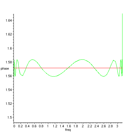
Equation 3. Second allpass filter, has 90 (+- 0.7) degrees relative phase to first filter over a long range of frequencies.
> plot({argument(H_1(exp(I*freq))), argument(H_2(exp(I*freq)))}, freq=0..Pi, phase = -Pi..Pi);
Figure 1. Phases of H_1 (green) and H_2 (red).
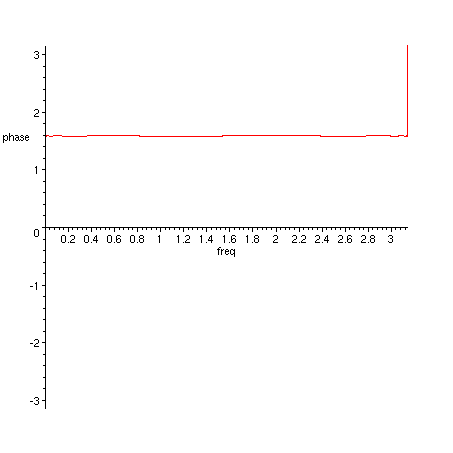
> plot(argument(H_2(exp(I*freq))/H_1(exp(I*freq))), freq=0..Pi, phase = -Pi..Pi);
Figure 2. Phase difference of H_2 and H_1.
> plot({argument(H_2(exp(I*freq))/H_1(exp(I*freq))), Pi/2}, freq=0..Pi, phase = Pi/2*0.95..Pi/2*1.05);
Figure 3. Phase difference of H_2 and H_1 (green), detail near 90 degrees (red).
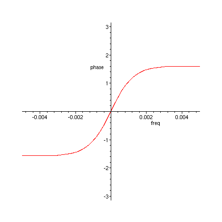
> plot(argument(H_2(exp(I*freq))/H_1(exp(I*freq))), freq=-0.005..0.005, phase = -Pi..Pi);
Figure 4. Phase difference of H_2 and H_1, detail near 0 Hz.
You can use the 90 degree phase difference of the filters as such, or you can construct a complex filter and analyze its properties:
> H := z -> 0.5*(H_2(z)+I*H_1(z));
Equation 4. Combined complex filter that will remove negative frequencies.
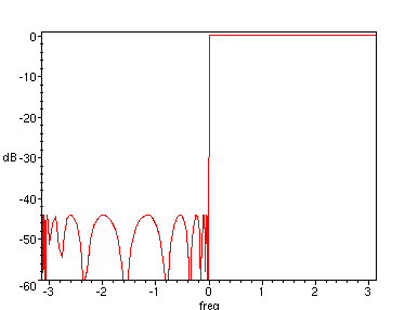
> plot(20*log10(abs(H(exp(I*freq)))), freq=-Pi..Pi, dB=-60..1, axes=boxed);
Figure 5. Frequency response of filter in Equation 4.
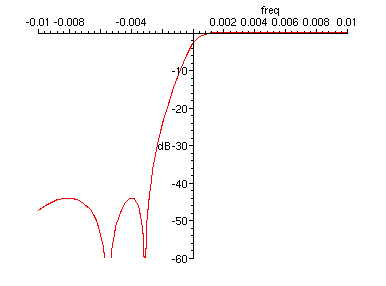
> plot(20*log10(abs(H(exp(I*freq), 0.4))), freq=-0.01..0.01, dB=-60..1);
Figure 6. Frequency response of filter in Equation 4, transition band detail
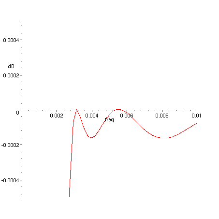
> plot(20*log10(abs(H(exp(I*freq), 0.4))), freq=0..0.01, dB=-0.0005..0.0005);
Figure 7. Frequency response of filter in Equation 4, transition band - passband detail.
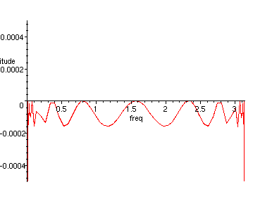
> plot(20*log10(abs(H(exp(I*freq)))), freq=0..Pi, magnitude=-0.0005..0.0005);
Figure 8. Frequency response of filter in Equation 4, passband detail
Transition bandwidth is 0.002 times the width of passband, stopband is attenuated down to -44 dB and passband ripple is 0.0002 dB.
Plenty cheap for a total of 8 multiplications (plus final scaling by 0.5)!
The coefficients were found using a generic evolutionary algorithm. I believe that it would be possible to design coefficients for this filter structure using the software by Artur Krukowski, which finds coefficients for halfband filters: http://www.cmsa.wmin.ac.uk/~artur/Poly.html
Update 2004/01/13
Ben Saucer has succesfully implemented this filter pair to be used in his audio effect. Here are some useful (edited) excerpts from our e-mail correspondence.
Here's a quick diagram of the allpass pair:
        ................ filter 1 .................
   +--> allpass --> allpass --> allpass --> allpass --> delay --> out1
   |
  in
   |    ................ filter 2 .................
   +--> allpass --> allpass --> allpass --> allpass ------------> out2 (+90 deg)
We can use cookbook formulas to convert an allpass section into code. A general IIR recurrence relation:
  out(t) = a0*in(t) + a1*in(t-1) + a2*in(t-2) + ...
         + b1*out(t-1) + b2*out(t-2) + ...
results in the transfer function:
         a0 + a1*z^-1 + a2*z^-2 + ...
  H(z) = ----------------------------
          1 - b1*z^-1 - b2*z^-2 - ...
The allpass section in question has the following transfer function:
          a^2 - z^-2
  H(z) = ------------
         1 - a^2 z^-2
We want to convert this into the recurrence relation. According to the cookbook formulas and the above transfer function:
  a0 = a^2, a2 = -1, b2 = a^2, rest of coefficients zero

  =>  out(t) = a^2*in(t) - in(t-2) + a^2*out(t-2)
which simplifies to the one-multiplication allpass section:
out(t) = a^2*(in(t) + out(t-2)) - in(t-2)
![[Maple Math]](http://yehar.com/blog/wp-content/uploads/2009/09/hilbert1.gif)


High quality stuff! I’ve used this filter for extracting audio envelopes as abs(out1)+abs(out2) and a peak-hold filter.
It would be interesting to learn more about the theory behind it, and how the coefficients were calculated. Krukowskis site appears to have been taken offline permanently =(
David, I don’t know well the theory behind this. Waybackmachine has some PDF’s at Artur Krukowski’s web page. The first of them cites harris, f., M. d’Oreye de Lantremange and A. G. Constantinides, “Digital signal processing with efficient polyphase recursive all-pass filters”, presented at International Conference on Signal Processing, Florence, Italy, September 4-6, 1991.
I too have used this for envelope extraction, as sqrt(out1^2+out2^2) followed by a smoothing filter. This formulation gives a flat envelope for any audio frequency sinusoid. I recall that there were some problems from the large group delay at low frequencies. Unfortunately I did not put here a phase plot to highlight that.
For calculation of the coefficients I used Differential Evolution optimization with a minmax cost function. It can be guided a bit by the fact that the a’s of the two filters are always interleaved. It is enough to look at one half of the spectrum, the other half will behave exactly the same. This symmetry is also reflected in the low amount of computations that the filters require, so it should not be broken even when requirements for the other half of the frequency response are more relaxed. It is better to keep the symmetrical structure.
Very nice blog!
The figure 1 doesn’t appear.
Thanks Harry,
figure 1 should be visible now
Great presentation! It would be interesting to compare this to the Hutchins design using six 1st order all-passes. E.g., as implemented in Csound:
http://www.csounds.com/manual/html/hilbert.html
http://sourceforge.net/p/csound/csound5-git/ci/08a709e36bd9911e99ec16d1677fa9c62d3c19b6/tree/Opcodes/ugsc.c#l92
hey Olli, first time i stumbled upon your blog. this pair of APFs to compute something like an analytic signal appears very useful (like for frequency shifting). i might put it to use someday.
i noticed your page on Wikipedia (small world). anyway, i might disagree with you about the Wikipedia editor “Bob K”. i *don’t* think he’s been as useful as he is prolific. i think he has crapped up many, many articles related to signal processing and the sampling theorem. but i’m glad to see you at the English wikipedia.
bestest,
r b-j
oh, BTW, were you (yehar) the person that had that old SHArC page on the web? does it still live somewhere?
Hi RBJ! I don’t have a SHARC page, and don’t remember having had one. Maybe a pile of documents in one dir but nothing more. By the way by some extra modulation trickery it is possible to run this filter back and forth to get a linear-phase negative frequency removal filter. All the best and see you around!
Thanks Olli for your explanations. I’m trying this Hilbert method to remove the negative frequencies to make a frequency shifter. Something is wrong and I’m not getting the desired results. Although it works when I use a FIR filter instead. I have a couple of questions:
1. What to do with the two outputs for those two allpass cascaded filters? Are they the imaginary part that should be mixed with the real input?
2. Why did you place a 1 sample delay after filter 1. It seams to me that this will introduce a zero at half the sampling rate. But I’m probably wrong.
I’m confused in many things so it would help if you shed some light. Thanks :)
Hello AM,
1. Do not use the real input as the real part. Use the output one of the filters as the real part and the output of the other filter as the imaginary part. See Eq. 4.
2. The one-sample delay will introduce a pole at z = 0 (and a zero at z=infinity). This is needed because the poles of the two filters must be in alternate order on the z-plane real axis to give the lowest possible ripple in the phase response difference between them. For each filter, the poles are located symmetrically on the right and left half-axis, and filter 2 has the innermost symmetrical pole pair. The extra pole in the filter 1 due to the delay goes between those poles.