If you have a problem where you need to find the optimal values for a set of real variables, try this library written by Magnus Jonsson and me.
opti.cpp opti.hpp- Optimization library v1.1
MersenneTwister.h - Mersenne Twister random number generator required by the library (by Rick Wagner)
optitest.cpp keyboard.h - Example program with keyboard IO routines
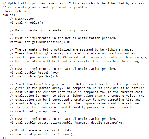
Look at opti.hppfor the interfaces to the library. Read this text to know what is the idea of the various things and what can be done to improve the optimization.
You must present your optimization problem in form of a cost function that accepts a vector of parameters (real numbers) and gives out a single (real) number. The library will then try to find the combination of values for the parameters that minimizes the value your cost function. Sometimes a sub-optimal solution is found, but, depending on the hardness of the problem, often the global optimum is reached.
The basic idea of how an evolutionary algorithm works is as follows. First a population of parameter vectors is initialized to random values that cover the whole range of possible values for the optimal solution. Then the evolutionary algorithm will combine members of the population to create new trial vectors. The trial vectors may replace inferior members in the population. Ultimately, the population will dive into a minimum, hopefully the global minimum, of the cost function.
Different evolutionary strategies available in the library:
Differential evolution (class DE)
This algorithm adds scaled-down differences between population members to other population members to create trial vectors.
G3PCX (class G3, PCX is the default recombinator)
This algorithm is based on creating trial vectors randomly in the vicinity of existing population members. The extent of the randomness depends on the scattering of the population.
In the library, the recombinator means the part of the evolutionary algorithm that combines population members to create the trial vectors. We made the library in a flexible way so that you can exchange the recombinators between the optimization strategies. A default recombinator is provided for each strategy, but some experimenting with the recombinator parameters may improve the reliability and the speed of the optimization, as different types of problems benefit from different approaches. The parameters in the recombinators are as follows.
DERecombinator
This recombinator is to be used with Differential Evolution. The parameter cr defines how many of the parameters from the trial vector will replace corresponding parameters in the inferior vector. Usually a value of 1 is OK, but if your population size is small, there is a danger that the dimensionality of your population might drop too low. A value of 0.999 will add a refreshing dash of randomness to the otherwise linear way of combining of the vectors, but will not disturb the over-all scheme too much. The parameter c is the number by which the difference between two population members is multiplied before it is added to another member to create the trial vector. Values such as 0.3, 0.4, 0.6, 0.7 and 0.8 have been useful.
PCXRecombinator
This recombinator is to be used with the G3 strategy. The parameter sd1 and sd2 are standard deviations of the random vectors that are created around existing population members, expressed relative to distances between randomly selected members of the populaton. It is fine to have the same value for both. 0.1 is a nice choice. You should normally stay under 1. A low number will make the population progress in smaller steps, thus better fine-tuning a found minimum, but a higher value will make the population explore more distant areas in the cost function. numparents means how many population members will be selected for the recombination process ecah time. 3 is the default value, which I haven't found useful to change.
The population size is something you must always define by yourself. Practical values are in the range of 30-1000, but even higher values might be used in over-night optimizations where you don't want to take any chances. If the population is large enough to explore the cost function properly, the global minimum will be reached within a low numerical error. You should always use more population members than you have dimensions in your problem.
The optimization is advanced by repeated calling of the evolve() function, which advances the population somewhat (how many evaluations of the cost function it does depends on the implementation of the strategy) and returns the cost of the best parameter vector so far in the population. Also the average cost of the population can be quickly retrieved using the avarageCost() function. The optimization should be stopped when there is no more progress within the numerical accuracy that you require. The best vector in the population is returned by the function best(). Try to refrain from printing progress information on each iteration, or your program might be occupied mostly by the print function...
If many repeated runs of the optimization return the same solution, it is quite likely that you have reached the global minimum, because there are typically a huge number of local minima and if you are stuck at one, you probably won't be stuck at the same the next time. Just look at the solved digits of the cost function value. These will work as a kind of fingerprint of the minimum. If you have problems getting into the global minimum or you are unsure that you are there, you may want to start with a similar problem but of a lower dimensionality. Then increase the dimensionality step by step. If you see a nice trend in the costs of the found solutions for each dimensionality, then this is an extra encouragement that you are at the global minimum.
To speed up things, reduce the running time of your cost function. If your cost function is a sum of a number of terms, then you can employ the compare variable passed to the cost function by the optimizer. If your cost seems to go above this value, then you can stop evaluation of the terms and just return compare or some larger number. This will instruct the optimizer that the evaluated trial vector is worse than another other vector it is comparing it against, and therefore can be discarded. If you use this trick, then it makes sense to first evaluate terms you suspect will give the biggest penalty.
It is also possible to constrain the variables being optimized. You can do this by modifying the input vector at the beginning of the cost function. But carefully consider what might be the consequences of this modification. If you hard-limit some parameters, will this reduce the dimensionality of your population as you set a parameter to the same value in many of the vectors? It can be better to just penalize strongly solutions that go outside your bounds of choice, by adding a large penalty term. Perhaps even create a sort of a funnel in the cost function that will direct astray vectors back on track. This can be done by penalizing according to the severity of the constraint violation.
This is getting a bit problem-specific, but if you are doing something like least mean square approximation, you typically are integrating the error function through sampling. Do this so that you concentrate more samples at the known problem areas of the function. This way you can reduce the total number of samples significantly and will speed up the execution of the cost function.