What would the M87* black hole image look like if we saw 230 GHz radio waves?

I originally posted this as a question and an answer on physics.stackexchange.com, but it was not received well there and was closed.

The Event Horizon Telescope (EHT) M87* black hole image is equivalent brightness temperature, $T_\mathrm{b}$, in Kelvins mapped to color using a perceptually uniform colormap from ehtplot. By Rayleigh–Jeans law, equivalent brightness temperature is proportional to specific intensity:

$$T_b = \frac{c^2}{2\nu^2k}I_\nu,\tag{1}$$

where $I_\nu$ is the specific intensity, $c$ is the speed of light, $\nu$ is the observing frequency (230 GHz), and $k$ is the Boltzmann constant (source: paper IV).

Based on the appearance of the black hole image, the lightness of the color per CIECAM02 color appearance model assumed to be perceptually uniform. Lightness does not fully define a color and allows to create arbitrarily customized colormaps such as the one used for the black hole image.

In perceptual photometry, radiant intensity $I_\mathrm{e}$ in watts per steradian (W/sr) is converted to luminous intensity $I_\mathrm{v}$ in candelas (cd) by:

$$I_\mathrm{v} = 683\,\overline{y}(\lambda)\,I_\mathrm{e},\tag{2}$$

where ${\overline {y}}(\lambda )$ is the standard luminosity function, which is zero-valued outside the visible spectrum (source: Wikipedia article on photometry).

Perhaps a more natural mapping of the monochromatic 230 GHz black hole image to a visible color image would be obtained by equating $I_\nu$ to $I_\mathrm{e}$, by replacing ${\overline {y}}(\lambda )$ of Eq. 2 by a non-zero value, and by creating an image that reproduces the luminous intensity $I_\mathrm{v}$, as if we were able to see 230 GHz radio waves. By "more natural" I mean that we have intuitive facilities for processing visual intensity as is, whereas in the published image, intensity was mapped to a perceptually uniform scale. Chromaticity could be left out by presenting a gray scale image. Question: What would the black hole image look like with such a colormap?

After obtaining the brightness temperature data, it could be converted from the linear intensity scale using the sRGB transfer function (from Wikipedia article on sRGB):

$$\gamma(u) = \begin{cases}12.92 u & u \lt 0.0031308 \\1.055 u^{1/2.4} - 0.055 & \text{otherwise,}\end{cases}\tag{3}$$

where $u$ is linear intensity, and saved in an image file for viewing.

One approach to obtain a brightness temperature image would be to invert (as in finding the inverse function) the colormap of the published image and to work from that. I downloaded the 16-bit/channel TIFF Fullsize Original eso1907a.tif obtained 2019-04-12 from ESO (they have since replaced the file with an 8-bit/channel TIFF, obtained 2019-04-14). There are a couple of things that make inverting the colormap difficult. Firstly, the image does not come with reliable information about the colormap, such as a colorbar. Secondly, the 16-bit/channel TIFF has 18992 unique colors (8-bit/channel TIFF has 67395), whereas I can only get 256 unique colors from pyplot.get_cmap('afmhot_u') in Python. This makes me believe that the image is not directly colormapped brightness temperature but has been altered afterwards, perhaps smoothed and/or contrast stretched. It is difficult to guess what processing might have taken place and in which color space, although the scientific nature of the image limits what would be responsibly done. An EXIF field shows that the image was saved with Adobe Photoshop CC 2019 (Windows), so the direct source is not a (Python) script. It is possible that just cropping or tagging was done in Photoshop. However, if we highlight the 10 % green channel contour and 50 % red channel contour of the 16-bit eso1907a.tif, most of the central shadow shows an inversion in the order of the contours, which means that the image is not directly from a colormap:

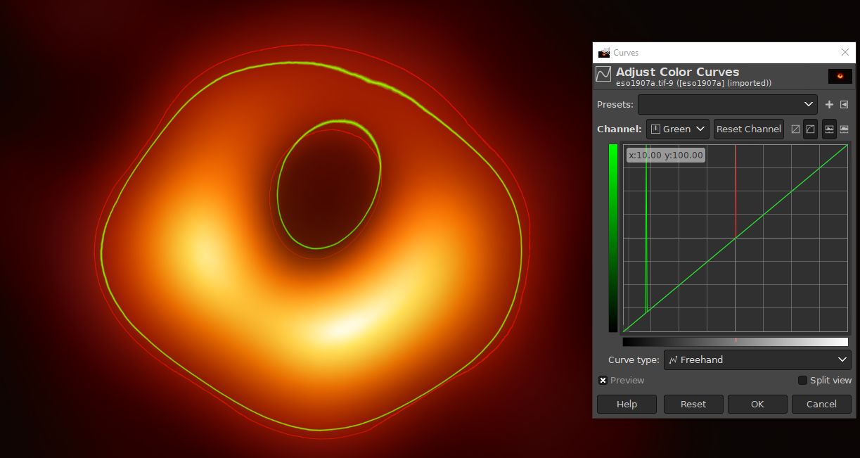
Figure 1. An analysis of 16-bit eso1907a.tif in GIMP by highlighting the contours in which the red color channel has 50 % value and the green color channel has 10 % value. Original image credit: Event Horizon Telescope.

Another approach would be to reconstruct the brightness temperature data from earlier data in the imaging pipelines. Katie Bouman's recent Caltech talk (published 2019-04-12) explains that the final image was a combination of images generated by three pipelines: DIFMAP, eht-imaging, and SMILI, each with an image from 2017-04-05, 06, 10, and 11, each image blurred so that they were similar enough as measured by normalized cross-correlation and all of the images averaged.

Based on this, there is yet another way to construct the final image, by averaging brightness temperatures of Fig. 15 of Paper IV:

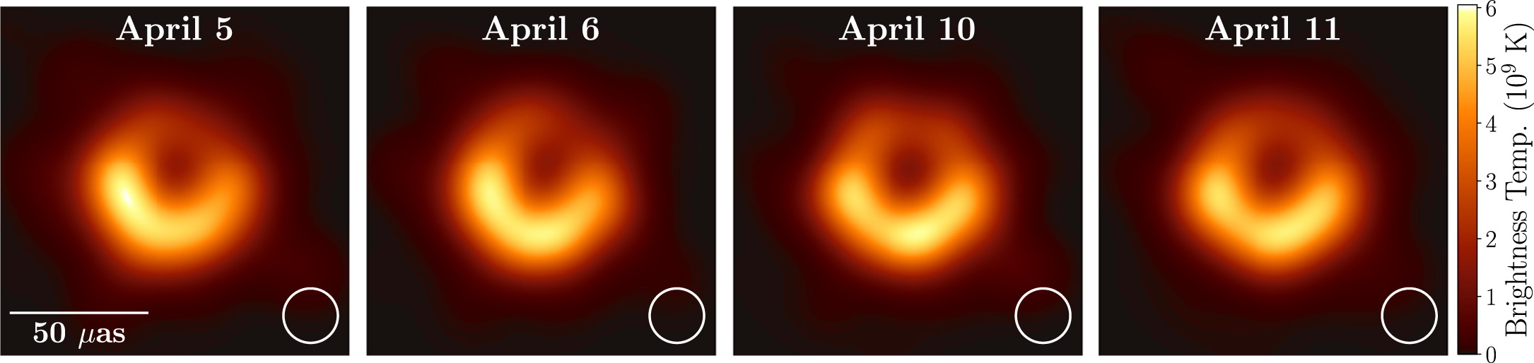
Figure 2. Fig. 15 of Paper IV. The subfigures are averages of blurred images from the three imaging pipelines. Image credit: Event Horizon Telescope.

Conveniently, the figure has a labeled colorbar. The image format is JPEG, so there will be at least some compression artifacts in addition to the white overlaying graphics. We can load the image and separate the color bar and the four images, and compare the color bar to afmhot_u, using Python script 1 below. The result:

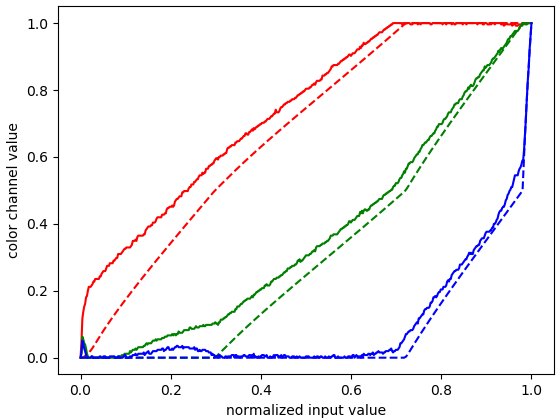
Figure 3. Red-green-blue (RGB) color channel values from the color bar of Fig. 2 (solid) and from the afmhot_u colormap (dashed), as function of normalized input value proportional to brightness temperature.

The knee points of the color channel curves (Fig. 3) of the color bar in Fig. 2 are approximately at the same input values as those of afmhot_u, which is further evidence that this colormap was used, but some knee points have been shifted horizontally. This could be some kind of an artifact from color space conversions with truncation of the red channel resulting in leakage to the other channels, but a proper interpretation of the shift is difficult. Because of the differences, an inversion of the afmhot_u colormap cannot be used.

Or one could ask the EHT imaging team for the brightness temperature data.

We can scrape the colormap from the colorbar in Fig. 2, convert each of its subfigures by picking for each pixel the brightness temperature that gives the least mean square error in the RGB triplet, average the brightness temperature subfigures, and save the result using the afmhot_u colormap (Fig. 4) and as intensity in sRGB using Eq. 3 (Fig. 5). This is done by Python script 2 below.

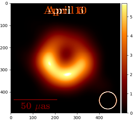
Figure 4. Brightness temperature (in units of $10^9$ K) of the reconstructed final black hole image colormapped using afmhot_u. Horizontal and vertical axis are in pixels of the same size as in Fig. 2. Processed from image credit: Event Horizon Telescope.

Figure 5. Brightness temperature of the reconstructed final black hole image saved as proportional intensity using the sRGB transfer function. Processed from image credit: Event Horizon Telescope.

The subfigures were assumed to be registered already beforehand. Horizontal registration may have slight additional error introduced by cropping of the original figure to subfigures at whole pixel resolution.

The reconstructed image in Fig. 4 looks quite similar to the published first black hole image, but the central shadow in the reconstructed image is not as pronounced.

The central shadow is even less pronounced in Fig. 5 which answers the question for now. EHT has since published the imaging pipelines, which should allow proper reproduction of the final brightness temperature image.

Python script 1

import io
from PIL import Image
import cv2
import urllib.request as urllib2
import matplotlib.pyplot as plt
import numpy as np
from scipy.misc import imshow
import ehtplot as eht
img = np.array(Image.open(io.BytesIO(urllib2.urlopen("https://iopscience-event-horizon.s3.amazonaws.com/2041-8205/875/1/L4/downloadHRFigure/figure/apjlab0e85f15_hr.jpg").read())))
bar = np.flip(img[9:502 , 2075:2076, :]/255, 0)
zero_to_almost_1 = [[j/255 for j in range(256)]]
afmhot_u_bar = np.delete(plt.get_cmap('afmhot_u')(zero_to_almost_1), 3, 2)
img1 = img[8:503, 0:494, :]/255
plt.imshow(img1)
plt.show()
img2 = img[8:503, 518+0:518+494, :]/255
plt.imshow(img2)
plt.show()
img3 = img[8:503, 518*2+1+0:518*2+1+494, :]/255
plt.imshow(img3)
plt.show()
img4 = img[8:503, 518*3+0:518*3+494, :]/255
plt.imshow(img4)
plt.show()
x_afmhot_u = np.array(range(256))/255
x_bar = np.array(range(bar.shape[0]))/(bar.shape[0]-1)
plt.plot(x_bar, bar[:,0,0], 'r-', x_afmhot_u, afmhot_u_bar[0,:,0], 'r--', x_bar, bar[:,0,1], 'g-', x_afmhot_u, afmhot_u_bar[0,:,1], 'g--', x_bar, bar[:,0,2], 'b-', x_afmhot_u, afmhot_u_bar[0,:,2], 'b--')
plt.ylabel('color channel value')
plt.xlabel('normalized input value')
plt.show()

import io

from PIL import Image

import cv2

import urllib.request as urllib2

import matplotlib.pyplot as plt

import numpy as np

from scipy.misc import imshow

import ehtplot as eht

img = np.array(Image.open(io.BytesIO(urllib2.urlopen("https://iopscience-event-horizon.s3.amazonaws.com/2041-8205/875/1/L4/downloadHRFigure/figure/apjlab0e85f15_hr.jpg").read())))

bar = np.flip(img[9:502 , 2075:2076, :]/255, 0)

zero_to_almost_1 = [[j/255 for j in range(256)]]

afmhot_u_bar = np.delete(plt.get_cmap('afmhot_u')(zero_to_almost_1), 3, 2)

img1 = img[8:503, 0:494, :]/255

plt.imshow(img1)

plt.show()

img2 = img[8:503, 518+0:518+494, :]/255

plt.imshow(img2)

plt.show()

img3 = img[8:503, 518*2+1+0:518*2+1+494, :]/255

plt.imshow(img3)

plt.show()

img4 = img[8:503, 518*3+0:518*3+494, :]/255

plt.imshow(img4)

plt.show()

x_afmhot_u = np.array(range(256))/255

x_bar = np.array(range(bar.shape[0]))/(bar.shape[0]-1)

plt.plot(x_bar, bar[:,0,0], 'r-', x_afmhot_u, afmhot_u_bar[0,:,0], 'r--', x_bar, bar[:,0,1], 'g-', x_afmhot_u, afmhot_u_bar[0,:,1], 'g--', x_bar, bar[:,0,2], 'b-', x_afmhot_u, afmhot_u_bar[0,:,2], 'b--')

plt.ylabel('color channel value')

plt.xlabel('normalized input value')

plt.show()

Python script 2

(continues Python script 1)

This isn't particularly optimized, but will be fine for one-off conversion.

import imageio
from mpl_toolkits.axes_grid1 import make_axes_locatable

def icmap(img):  # inverse colormap
    h = img.shape[0]
    w = img.shape[1] 
    result = np.zeros((h, w))
    for y in range(h):
        for x in range(w):
            val = img[y, x]
            best_i = 0
            last_best_i = 0
            best_err = 3
            for i in range(bar.shape[0]):
                err = (val[0] - bar[i,0,0])**2 + (val[1] - bar[i,0,1])**2 + (val[2] - bar[i,0,2])**2
                if err < best_err:
                    best_i = i
                    best_err = err
                if err == best_err:
                    last_best_i = i
            result[y, x] = (best_i + last_best_i)/2
    return result

def to_sRGB(img):  # convert intensity 0..1 inclusive to uint8 0..255 inclusive with sRGB transfer function
    h = img.shape[0]
    w = img.shape[1] 
    result = np.zeros((h, w), dtype=np.uint8)
    for y in range(h):  # this will take time
        for x in range(w):
            if img[y, x] < 0.0031308:  # linear intensity to sRGB transfer function
                result[y, x] = ((12.92*img[y, x])*255 + 0.5).astype(np.uint8)
            else:
                result[y, x] = ((1.055*img[y, x]**(1/2.4) - 0.055)*255 + 0.5).astype(np.uint8)
    return result

bt1 = icmap(img1)  # This will take time...
bt2 = icmap(img2)
bt3 = icmap(img3)
bt4 = icmap(img4)
np.savetxt("bt1.csv", bt1, delimiter=",")  # Save for later reference
np.savetxt("bt2.csv", bt2, delimiter=",")
np.savetxt("bt3.csv", bt3, delimiter=",")
np.savetxt("bt4.csv", bt4, delimiter=",")
bt_average = (bt1+bt2+bt3+bt3)/4/(bar.shape[0]-1)*6  # Paper IV Fig. 15 colorbar max = 6
peak = np.max(bt_average[100:-100, 100:-100])  # Normalize based on the part of the image not polluted by overlays
bt_average_normalized = np.clip(bt_average/peak, 0, 1)*255/256
np.savetxt("bt_average.csv", bt_average, delimiter=",")
ax = plt.subplot(111)
im = ax.imshow(np.clip(bt_average, 0, peak), cmap='afmhot_u', vmin=0, vmax=peak)
divider = make_axes_locatable(ax)
cax = divider.append_axes("right", size="5%", pad=0.05)
plt.colorbar(im, cax=cax)
plt.savefig('bt_average_afmhot_u.png')
plt.show()
bt_average_sRGB = to_sRGB(bt_average_normalized)  
imageio.imwrite('bt_average_sRGB.png', bt_average_sRGB)

import imageio

from mpl_toolkits.axes_grid1 import make_axes_locatable

def icmap(img): # inverse colormap

h = img.shape[0]

w = img.shape[1]

result = np.zeros((h, w))

for y in range(h):

for x in range(w):

val = img[y, x]

best_i = 0

last_best_i = 0

best_err = 3

for i in range(bar.shape[0]):

err = (val[0] - bar[i,0,0])**2 + (val[1] - bar[i,0,1])**2 + (val[2] - bar[i,0,2])**2

if err < best_err:

best_i = i

best_err = err

if err == best_err:

last_best_i = i

result[y, x] = (best_i + last_best_i)/2

return result

def to_sRGB(img): # convert intensity 0..1 inclusive to uint8 0..255 inclusive with sRGB transfer function

h = img.shape[0]

w = img.shape[1]

result = np.zeros((h, w), dtype=np.uint8)

for y in range(h): # this will take time

for x in range(w):

if img[y, x] < 0.0031308: # linear intensity to sRGB transfer function

result[y, x] = ((12.92*img[y, x])*255 + 0.5).astype(np.uint8)

else:

result[y, x] = ((1.055*img[y, x]**(1/2.4) - 0.055)*255 + 0.5).astype(np.uint8)

return result

bt1 = icmap(img1) # This will take time...

bt2 = icmap(img2)

bt3 = icmap(img3)

bt4 = icmap(img4)

np.savetxt("bt1.csv", bt1, delimiter=",") # Save for later reference

np.savetxt("bt2.csv", bt2, delimiter=",")

np.savetxt("bt3.csv", bt3, delimiter=",")

np.savetxt("bt4.csv", bt4, delimiter=",")

bt_average = (bt1+bt2+bt3+bt3)/4/(bar.shape[0]-1)*6 # Paper IV Fig. 15 colorbar max = 6

peak = np.max(bt_average[100:-100, 100:-100]) # Normalize based on the part of the image not polluted by overlays

bt_average_normalized = np.clip(bt_average/peak, 0, 1)*255/256

np.savetxt("bt_average.csv", bt_average, delimiter=",")

ax = plt.subplot(111)

im = ax.imshow(np.clip(bt_average, 0, peak), cmap='afmhot_u', vmin=0, vmax=peak)

divider = make_axes_locatable(ax)

cax = divider.append_axes("right", size="5%", pad=0.05)

plt.colorbar(im, cax=cax)

plt.savefig('bt_average_afmhot_u.png')

plt.show()

bt_average_sRGB = to_sRGB(bt_average_normalized)

imageio.imwrite('bt_average_sRGB.png', bt_average_sRGB)

License

All images are licensed under the Creative Commons Attribution 4.0 International (CC BY 4.0).

References

The Event Horizon Telescope Collaboration, Kazunori Akiyama, Antxon Alberdi, Walter Alef, Keiichi Asada, Rebecca Azulay, Anne-Kathrin Baczko, David Ball, Mislav Baloković, John Barrett, Dan Bintley, Lindy Blackburn, Wilfred Boland, Katherine L. Bouman, Geoffrey C. Bower, Michael Bremer, Christiaan D. Brinkerink, Roger Brissenden, Silke Britzen, Avery E. Broderick, Dominique Broguiere, Thomas Bronzwaer, Do-Young Byun, John E. Carlstrom, Andrew Chael, Chi-kwan Chan, Shami Chatterjee, Koushik Chatterjee, Ming-Tang Chen, Yongjun Chen (陈永军), Ilje Cho, Pierre Christian, John E. Conway, James M. Cordes, Geoffrey B. Crew, Yuzhu Cui, Jordy Davelaar, Mariafelicia De Laurentis, Roger Deane, Jessica Dempsey, Gregory Desvignes, Jason Dexter, Sheperd S. Doeleman, Ralph P. Eatough, Heino Falcke, Vincent L. Fish, Ed Fomalont, Raquel Fraga-Encinas, William T. Freeman, Per Friberg, Christian M. Fromm, José L. Gómez, Peter Galison, Charles F. Gammie, Roberto García, Olivier Gentaz, Boris Georgiev, Ciriaco Goddi, Roman Gold, Minfeng Gu (顾敏峰), Mark Gurwell, Kazuhiro Hada, Michael H. Hecht, Ronald Hesper, Luis C. Ho (何子山), Paul Ho, Mareki Honma, Chih-Wei L. Huang, Lei Huang (黄磊), David H. Hughes, Shiro Ikeda, Makoto Inoue, Sara Issaoun, David J. James, Buell T. Jannuzi, Michael Janssen, Britton Jeter, Wu Jiang (江悟), Michael D. Johnson, Svetlana Jorstad, Taehyun Jung, Mansour Karami, Ramesh Karuppusamy, Tomohisa Kawashima, Garrett K. Keating, Mark Kettenis, Jae-Young Kim, Junhan Kim, Jongsoo Kim, Motoki Kino, Jun Yi Koay, Patrick M. Koch, Shoko Koyama, Michael Kramer, Carsten Kramer, Thomas P. Krichbaum, Cheng-Yu Kuo, Tod R. Lauer, Sang-Sung Lee, Yan-Rong Li (李彦荣), Zhiyuan Li (李志远), Michael Lindqvist, Kuo Liu, Elisabetta Liuzzo, Wen-Ping Lo, Andrei P. Lobanov, Laurent Loinard, Colin Lonsdale, Ru-Sen Lu (路如森), Nicholas R. MacDonald, Jirong Mao (毛基荣), Sera Markoff, Daniel P. Marrone, Alan P. Marscher, Iván Martí-Vidal, Satoki Matsushita, Lynn D. Matthews, Lia Medeiros, Karl M. Menten, Yosuke Mizuno, Izumi Mizuno, James M. Moran, Kotaro Moriyama, Monika Moscibrodzka, Cornelia Müller, Hiroshi Nagai, Neil M. Nagar, Masanori Nakamura, Ramesh Narayan, Gopal Narayanan, Iniyan Natarajan, Roberto Neri, Chunchong Ni, Aristeidis Noutsos, Hiroki Okino, Héctor Olivares, Tomoaki Oyama, Feryal Özel, Daniel C. M. Palumbo, Nimesh Patel, Ue-Li Pen, Dominic W. Pesce, Vincent Piétu, Richard Plambeck, Aleksandar PopStefanija, Oliver Porth, Ben Prather, Jorge A. Preciado-López, Dimitrios Psaltis, Hung-Yi Pu, Venkatessh Ramakrishnan, Ramprasad Rao, Mark G. Rawlings, Alexander W. Raymond, Luciano Rezzolla, Bart Ripperda, Freek Roelofs, Alan Rogers, Eduardo Ros, Mel Rose, Arash Roshanineshat, Helge Rottmann, Alan L. Roy, Chet Ruszczyk, Benjamin R. Ryan, Kazi L. J. Rygl, Salvador Sánchez, David Sánchez-Arguelles, Mahito Sasada, Tuomas Savolainen, F. Peter Schloerb, Karl-Friedrich Schuster, Lijing Shao, Zhiqiang Shen (沈志强), Des Small, Bong Won Sohn, Jason SooHoo, Fumie Tazaki, Paul Tiede, Remo P. J. Tilanus, Michael Titus, Kenji Toma, Pablo Torne, Tyler Trent, Sascha Trippe, Shuichiro Tsuda, Ilse van Bemmel, Huib Jan van Langevelde, Daniel R. van Rossum, Jan Wagner, John Wardle, Jonathan Weintroub, Norbert Wex, Robert Wharton, Maciek Wielgus, George N. Wong, Qingwen Wu (吴庆文), André Young, Ken Young, Ziri Younsi, Feng Yuan (袁峰), Ye-Fei Yuan (袁业飞), J. Anton Zensus, Guangyao Zhao, Shan-Shan Zhao, Ziyan Zhu, Joseph R. Farah, Zheng Meyer-Zhao, Daniel Michalik, Andrew Nadolski, Hiroaki Nishioka, Nicolas Pradel, Rurik A. Primiani, Kamal Souccar, Laura Vertatschitsch, and Paul Yamaguchi, "First M87 Event Horizon Telescope Results. IV. Imaging the Central Supermassive Black Hole", 2019 ApJL 875 L4, DOI: 10.3847/2041-8213/ab0e85. ("Paper IV").

Python script 1

Python script 2

License

References

Leave a Reply Cancel reply