
This article describes approaches for efficient isotropic two-dimensional convolution with disc-like and arbitrary circularly symmetric convolution kernels, and also discusses lens blur effects.
Keywords: depth of field, circle of confusion, bokeh, circular blur, lens blur, hexagonal blur, octagonal blur, real-time, DOF
Gaussian function approach
The circularly symmetric 2-d Gaussian kernel is linearly separable; the convolution can be split into a horizontal convolution followed by a vertical convolution. This makes 2-d Gaussian convolution relatively cheap, computationally, and "Gaussian blur" has become, partially for this reason, a popular operation in image processing. No other circularly symmetric (isotropic) convolution kernel is linearly separable. Usually a Gaussian kernel is real-valued. However, we can parameterize it with a complex number to obtain a complex 2-d Gaussian function that still satisfies conditions for separability and is circularly symmetric. This section of the article shows that the real part of weighted sums of such separable 2-d kernels can produce arbitrary 2-d circularly symmetric kernels. Special focus is given to implementation of circular blur, or convolution with a solid disk, which is useful for simulation of bokeh (circle of confusion) of camera lenses with fully open apertures.

A horizontal convolution followed by a vertical convolution (or in the opposite order) by 1-d kernels $f(x)$ and $f(y)$ effectively gives a 2-d convolution by 2-d kernel $f(x)\times f(y)$. To produce separable circularly symmetric 2-d convolution, the condition that must be satisfied for all $(x, y)$ is $f(\sqrt{x^2+y^2})\times f(0) = f(x)\times f(y)$. The right side of the equation is the 2-d kernel. The left side can be understood as taking a horizontal slice $f(x)\times f(0)$ of the kernel at $y=0$ and substituting $x\to r$ in the slice function to obtain a function $f(r)\times f(0)$ of radius $r = \sqrt{x^2+y^2}$ which the circularly symmetric kernel must be equal to at all $(x, y)$. If we assume that the 1-d kernels are normalized by $f(0)=1$, then the constraint for circular symmetry simplifies to $f(\sqrt{x^2+y^2}) = f(x)\times f(y)$. We will work with that simplifying assumption.
For starters, let's treat magnitude and phase of the complex kernels separately. The circular symmetry condition may be broken down into a magnitude condition and a phase condition that must both be satisfied. The magnitude condition reads $|f(\sqrt{x^2+y^2})| = |f(x) \times f(y)| = |f(x)|\times|f(y)| $, meaning that the kernel must have a Gaussian function as its magnitude function. Because in multiplication of complex numbers the phases are summed, the phase (argument) condition reads $\theta(\sqrt{x^2+y^2}) = \theta(x)+\theta(y)$, modulo $2\pi$, with the shorthand $\theta(x) = \arg(f(x))$. The only family of phase functions to satisfy this is $\theta(x) = a x^2$. The kernel function can be constructed as the product of a real Gaussian function, here called the envelope, and a complex phasor with $x^2$ as its argument. In one dimension these kernels have the form $e^{-a x^2} e^{i b x^2} = e^{- a x^2 + i b x^2} = e^{(- a + b i) x^2}$, where $i$ is the imaginary unit, $x$ is the spatial coordinate, $a$ is the spatial scaling constant of the envelope, and $b$ is the spatial scaling constant of the complex phasor. In two dimensions the form is $e^{- a x^2 + i b x^2} e^{- a y^2 + i b y^2} = e^{- a (x^2 + y^2) + i b (x^2 + y^2)} = e^{(- a + b i) (x^2 + y^2)}$, $y$ being the coordinate in the other dimension. These forms are not normalized to preserve average intensity in image filtering, but to give a value of 1 for $x = 0, y = 0$. Let's see what these look like.
 |
 |
|
 |
 |
|
Arbitrary circularly symmetric shapes can be constructed by a weighted sum of the real parts and imaginary parts of complex phasors of different frequencies. Fourier series is the standard approach for such designs. These give a repetitive pattern, but the repeats could be diminished by adjusting the spatial scale of the envelope. As necessary, sloping of the envelope can be compensated for in the weights of the sum, but simultaneous optimization of both will give the best results, as it can take advantage of that the envelopes need not be the same for each of the component kernels.
Let's try a 5-component square wave approximation, designed manually with the Fourier series applet of Paul Falstad.
 |
 |
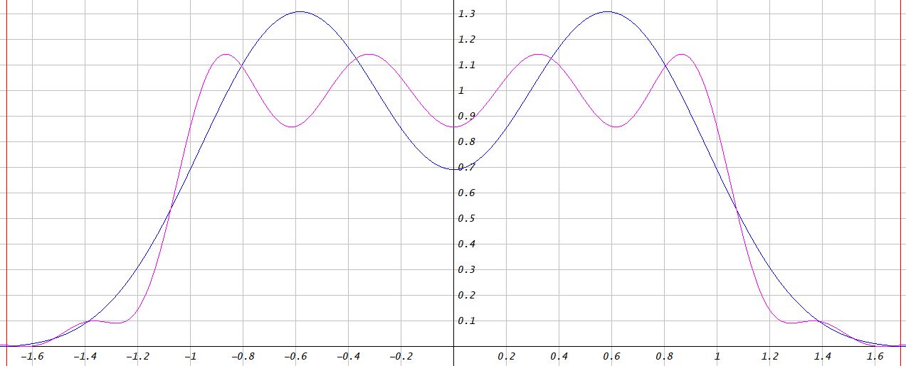
The formula for this series is $0.54100\ +\ 0.66318\ \cos(x)\ -\ 0.20942\ \cos(3 x)\ +\ 0.10471\ \cos(5 x)\ -\ 0.08726\ \cos(7 x)$. A bit of scaling (by 0.9) and shifting (by -0.01) was then done to make the ripples go evenly around the zero level and to avoid values greater than 1.
This is a pretty good indicator of the capabilities of this approach. The weighted component kernels were:
 |
 |
 |
 |
 |
By lowering the spatial scale of the magnitude part of each component kernel, one gets a result like this:

Not so bad! The halos would need to be eliminated, and the disk is also fading a bit toward the edges.
I searched for better circular kernels by global optimization with an equiripple cost function, with the number of component kernels and the transition bandwidth as the parameters. Transition bandwidth defines how sharp the edge of the disk is. The sharper it is, the more ringing there will be both inside and outside the disk. A transition bandwidth setting of 1 means that the width of the transition is as large as the radius of the disk inside. Below, 1-d component kernel formulas are given for a pass band spanning $x \in -1..1$ and a dual stop band spanning $ x\ \in\ -1.2\ ..\ -1\ \cup\ 1\ ..\ 1.2$.
 |
 |
 |
 |
 |
 |
 |
|


 |
|
|


The last one of the above, with 5 component kernels, is good enough for most practical applications as the ripple is as small as 1/250, about as much as the least significant bit for 8-bits-per-channel graphics, so invisible in almost all situations. As the number of components is increased, the components have an increasingly large weighted amplitude, as much as 36 times their sum for the 5-component system. This may become a practical problem if one aims for convolution kernel shapes with sharp transitions. A construction via Fourier series would probably give better-behaving components, but require more components than abusing the Gaussian envelope for ripple control as seems to be the case in the above given composite kernels.
Here's a bonus, with 6 components:

The 1-d composite kernel can be truncated to range $x \in -(\textrm{pass band radius + transition bandwidth}\ ..\ \textrm{pass band width + transition bandwidth})$. This only necessitates a stop band equiripple condition for $|x| \in \textrm{pass band radius + transition bandwidth}\ ..\ \sqrt{2}(\textrm{pass band radius+ transition bandwidth})$ to ensure a flat stop band in the corners of the 2-d convolution kernel square. However, at least for up to the above given 5th order composite kernel, the stop band ripples start to slope out already within that range, so no savings can be made.
Let's see the 5-component circular blur in action.
 |
|
 |
 |
 |
 |
 |
 |
The circular blur here is the weighted sum of the real and imaginary parts of the 5 component convolutions.
Let's try another image, one which will better show the blur disks.
 |
 |
 |
 |
Looks like an out-of-focus camera, doesn't it?
Recursive approximations
The examples presented above were done with 1-d finite impulse response (FIR) filters of which I now have a FFT-based implementation. More efficient would be to use identical pairs of complex 1-d causal and anti-causal infinite impulse response (IIR) filters to achieve a symmetric composite filter. Early results:
 |
|
The above first attempt filter is quite heavy, about 110 complex multiplications (some of which involve real numbers) per color channel per pixel. But it is independent of the size of the blur (disregarding boundary conditioning that may add a penalty proportional to the radius times the number of edge pixels in the image).
Perhaps circular blur is not the best use for the phased Gaussian kernels, as no sharp edges can be achieved. How about constructing an airy disc for anisotropic low-pass filtering of the image in a manner that gives an equal upper frequency limit for features in diagonal, horizontal, vertical, or any direction? Food for thought... Update: yes, it works
Updates
There are now GPU implementations of this method out there. Kleber Garcia gave a SIGGRAPH 2017 talk (accompanying conference paper) about his 1 and 2-component blur implementations. They can be seen at work in FIFA 17 screenshots. The talk inspired Bart Wronski to write a Shadertoy implementation, with an accompanying text. Kleber Garcia responded with his own Shadertoy implementation.
I have also gained more understanding of the math involved. Each 1-d component kernel is really just a Gaussian function, but with a complex width parameter. The original condition I wrote for separability demands that A) the 2-d convolution kernel is a circularly symmetrical revolution of the 1-d kernel (the value of the 2-d kernel at radius $r$ equals the 1-d kernel at position $r$), B) the same coefficients are used for the horizontal and the vertical 1-d kernels. Then the final output for each component is a weighted sum of the real and imaginary parts of the 2-d convolution (implemented as a horizontal and a vertical 1-d convolution) result. The weighed sum with a weight $a$ for the real part and a weight $b$ for the imaginary part can be seen as complex multiplication by $a-bi$ followed by discarding of the imaginary part. If we modify requirement A to: "the 2-d convolution kernel is circularly symmetrical", then we can absorb the said multiplication into the 1-d convolution kernel by multiplying each coefficient by the complex number $\sqrt{a-bi}$. Because we have two 1-d convolution passes, that number will be squared, hence the square root. Now we have coefficient-wise identical horizontal and vertical 1-d convolutions that produce a 2-d convolution with a kernel that is circularly symmetrical. The work saved is that we don't need to calculate (or store!) the imaginary output of the 2nd 1-d convolution, because only the real part of its result will be used.
Having done this optimization, the 1-d kernel can be expressed (recycling variable names) simply as $(c+di)e^{(a + b i) x^2} = e^{ax^2}\big(c\cos(bx^2) - d\sin(bx^2)\big) + ie^{ax^2}\big(d\cos(bx^2) + c\sin(bx^2)\big),$ resulting in a 2-d kernel $(c+di)^2e^{(a+bi)(x^2+y^2)}.$ One can then globally optimize the coefficients $(a, b, c, d)$ of a horizontal slice $(c+di)^2e^{(a+bi)x^2}$ (note the square) of the 2-d kernel to get a desired shape of the real part $e^{ax^2}\big((c^2 - d^2)\cos(bx^2) - 2cd\sin(bx^2)\big)$ of the slice, or the sum of these from multiple components.
Using this notation, the $(a, b, c, d)$ coefficients are obtained from the old coefficients $(a, b, r, i)$, where $r$ and $i$ are the weights of the real and the imaginary part of the component:
a = -a;
b = b;
c = sqrt(2)*(sqrt(r*r + i*i) + r)*sqrt(sqrt(r*r + i*i) - r)/(2*i);
d = -sqrt(2)*sqrt(sqrt(r*r + i*i) - r)/2;

// Use these coefs as:
// real_coef = (c*cos(x*x*a) - d*sin(x*x*a)) * exp(b*x*x);
// imag_coef = (d*cos(x*x*a) + c*sin(x*x*a)) * exp(b*x*x);

// a, b, c, d:
// 1-component
-0.8623250000, 1.6248350000, 1.1793828124, -0.7895320249
// 2-component
-0.8865280000, 5.2689090000, -0.7406246191, -0.3704940302
-1.9605180000, 1.5582130000, 1.5973700402, -1.4276936105
// 3-component
-2.1764900000, 5.0434950000, -1.4625695191, -0.7197739911
-1.0193060000, 9.0276130000, -0.1480093005, -0.5502424493
-2.8151100000, 1.5972730000, 2.2293886172, -2.3101178772
// 4-component
-4.3384590000, 1.5536350000, 4.5141678065, -5.1132787901
-3.8399930000, 4.6931830000, -3.7350649493, -2.0384600009
-2.7918800000, 8.1781370000, 0.0866540887, -1.7480940853
-1.3421900000, 12.3282890000, 0.3569701172, -0.3426757426
// 5-component
-4.8926080000, 1.6859790000, 5.7626795783, -7.4542110865
-4.7118700000, 4.9984960000, -6.4033389291, -2.2547313456
-4.0527950000, 8.2441680000, -0.2167382954, -3.6413223544
-2.9292120000, 11.9008590000, 1.0940793322, -0.8300714338
-1.5129610000, 16.1163820000, -0.3717954486, -0.0134482550
// 6-component
-5.1437780000, 2.0798130000, 5.2941931370, -10.5050024737
-5.6124260000, 6.1533870000, 10.9927011254, -2.6383360349
-5.9829210000, 9.8028950000, -10.1550051566, -7.9777845753
-6.5051670000, 11.0592370000, 4.8737688428, -9.7488280697
-3.8695790000, 14.8105200000, -1.6383505756, -1.1306841329
-2.2019040000, 19.0329090000, -0.1309780866, -0.4122368969
Negative values in the 2-d convolution kernel may be off-putting, because they create a cheap-looking sharpening kind of effect. I optimized some low component count coefficient sets that give almost no negative values in the 2-d convolution kernel:
// a, b, c, d
// 1-component, stp-band maximum = 0.3079699786
-2.0126256644, 1.0462519386, 1.7772360464, -1.5705215513
// 2-component, stop-band maximum = 0.1422940279
-1.8755934460, 5.6868281810, -1.1341154250, -0.4727562391
-3.0859247607, 0.0311853116, 14.9843211153, -14.9911604837
As noted by Bart Wronski, in addition to solid discs, also donuts may be desirable bokeh shapes. Donuts are associated at least with large focal length mirror lenses. It would probably be possible to optimize the components to get a visually impressive sharp donut, sharper than the discs shown. I did some experiments about that, but it didn't look very nice.
For approximation of general 2-d (or 3-d) kernels that do not need to be circularly symmetric, as sums of separable 2-d convolutions, see Treitel, S. & Shanks, J. (1971). The design of multistage separable planar filters. IEEE Transactions on Pattern Analysis and Machine Intelligence, 9(1), 10–27.
Circular blur using prefix sums and summed area tables
Circular blur done using the phased gaussian kernels is not perfect because it has the transition band. A completely different approach would be to calculate each blurred output pixel separately by summing the pixels that fall within the disk radius from the position of the pixel. There is a very efficient way to do this. The area of the disk can be subdivided into a minimum number of rectangular pieces and a summed area table can be used to efficiently calculate the sum of pixels within each rectangle. Here is an illustration of the idea:

Kyle McDonald has been working on the same problem and shows a more efficient packing with his Processing application:

A somewhat simpler way would be to subdivide the circle into one-pixel-height strips. The sum of the pixel values of a strip could be calculated from the prefix sum over the length of each column, requiring only two lookups per strip. The number of rows would be roughly the diameter of the circle, and the number of lookups roughly four times the radius, or $4r$.
By combining the use of summed area tables and horizontal and vertical prefix sums we get a rather boring-looking hybrid approach that appears to be the most efficient:

For large $r$, the hybrid approach takes about $(8-4\sqrt{2})r \approx 2.34\ r$ lookups: 4 for the rectangle (from a summed area table) but dominated for large $r$ by 2 for each stripe (from horizontal or vertical prefix sum). In comparison, Kyle McDonald's approach takes about $(12-4\sqrt{5})r \approx 3.06\ r$ table lookups with both summed area tables and prefix sums available and about $(16-\frac{24\sqrt{5}}{5})r \approx 5.27\ r$ table lookups with only the summed area table available. The latter result is identical for the hybrid approach. If the whole image is convolved with a disc of constant radius, the center rectangle in the hybrid approach can be done with a constant complexity box blur and a summed area table will not be needed, relieving requirements for the bit depth used in the calculations.
To get an anti-aliased edge for the circle, the edge pixels can be summed or subtracted with weights separately, doable in the ready-for-prefix-sum representation. The number of pixels that should receive anti-aliasing is about $(4\sqrt{2} + 16 - \frac{24\sqrt{5}}{5})r \approx 10.9\ r$, increasing the total cost of the algorithm to $(24 - \frac{24\sqrt{5}}{5})r \approx 13.27\ r$. Each weight will be shared by 8 edge pixels, which may give some computational savings. In conclusion, anti-aliased or not, the complexity of this way of blurring will be proportional to the radius of the disc times the number of pixels in the image. The decompositions (lookup recipes) of different size blurs could be stored in tables, which would allow also the use of a depth map to blur different parts of the image with a different disk size.
Alternatively to exact antialising, one could approximate the longer monotonic antialias gradations as linear, by use of two horizontal prefix sum passes in series and two vertical prefix sum passes in series. The slope of each linear section would be thrown in first, then after calculation of the first prefix sum, the constant term of the linear section would be added, along with a value that terminates the section. Either of these would coincide with the values that define where the flat section of the disc starts for that horizontal or vertical stripe. The method could be made more accurate by increasing the number of linear sections, perhaps up to two per monotonous gradation.
If different size blurs are used in the same image, then one decision must be made on how the result should look: whether the blur scatters or gathers. Let's demonstrate with a square box blur, increasing the blur size towards the top of the image:
 |
 |
 |
With a variable blur kernel, scattering blur is more correct, because it preserves average image intensity, unlike gathering blur. With smooth blur size gradations, gathering blur should also look okay.
If the kernel is constant, blurring can be described mathematically by convolution of the input image by the blur kernel: $o = i*K$, where $o$ is the output image, $i$ is the input image and $K$ is the blur kernel. There are two ways to directly implement the convolution: In the scattering way, first the output image is cleared to zero, and then for each input pixel, a copy of the kernel $K$ is multiplied by the intensity of the input pixel, spatially shifted to the position of the input pixel, and added to the output image. In the gathering way each output pixel is formed by shifting a copy of the kernel reversed along each axis, to the position of the output pixel, and setting the output pixel to the sum of products of the pixel intensities in the shifted and reversed kernel and the input image. If the same kernel is used throughout the image, both ways of doing convolution will be identical. But if the size of the blur varies, we must acknowledge whether we do a scattering or a gathering convolution by $K$. We denote these by $\hat{*}$ for a scattering and $\check{*}$ for a gathering convolution by the variable kernel. The mnemonic is that the arrowhead points away to indicate scattering.
We define the order of calculation of written formulas to be from left to right with the exception that multiplication and convolution are calculated first and addition and subtraction last. The convolution operator $*$ has the following algebraic properties :
- Commutativity: $A*B = B*A$
- Associativity: $A*B*C = A*(B*C)$
- Distributivity: $A*C+B*C = (A+B)*C$
- Associativity with scalar multiplication: $a(A*B) = aA*B = A*(aB)$, where $a$ is a constant.
With scattering convolution $\hat{*}$ and gathering convolution $\check{*}$ by a variable kernel we have a drastically limited set of algebraic properties:
- Distributivity: $A\ \hat{*}\ C+B\ \hat{*}\ C = (A+B)\ \hat{*}\ C$ for scattering convolution and $A\ \check{*}\ C+B\ \check{*}\ C = (A+B)\ \check{*}\ C$ for gathering convolution.
- Distributivity, again: $C\ \hat{*}\ A+C\ \hat{*}\ B = C\ \hat{*}\ (A+B)$ for scattering convolution and $C\ \check{*}\ A+C\ \check{*}\ B = C\ \check{*}\ (A+B)$ for gathering convolution. This can be used for simplification of the calculation if both A and B are sparse, because then (A+B) will also be sparse and some coincident values may cancel.
- Associativity with scalar multiplication: $a(A\ \hat{*}\ B) = aA\ \hat{*}\ B = A\ \hat{*}\ (aB)$ for scattering convolution and $a(A\ \check{*}\ B) = aA\ \check{*}\ B = A\ \check{*}\ (aB)$ for gathering convolution.
When utilizing a summed area table, the constant-kernel calculation can be written as: $o = i*S_{xy}*K_{xy} = i*K_{xy}*S_{xy}$, where $o$ is the output image, $i$ is the input image, $S_{xy}$ is such a function that convolution with it gives the summed area table, and $K_{xy}$ is the sparse representation of the blur kernel that gives the blur kernel if convolved with $S_{xy}$ (or vice versa). It turns out that with a variable blur kernel, scattering convolution requires the scattering-friendly order of calculation: $o = i\ \hat{*}\ K_{xy}*S_{xy}$, and gathering convolution the gathering-friendly order $o = i*S_{xy}\ \check{*}\ K_{xy}$. Using the wrong order with a variable blur kernel would give rather unpredictable results and is not recommended. As a rule, if the kernel is not constant, scattering convolution should operate directly on the input image and gathering convolution should not be followed by further convolutions.
The computational complexity of the whole calculation is independent of the order of convolutions. Convolving something with $S_{xy}$ is cheap. It is also cheap to convolve something with $K_{xy}$, because it is sparse, that is, zero in all but a few places, amounting to a sum of shifted copies of the function that is being convolved. Rather than discussing the number of table lookups, the computational complexity of the blur can be described by the number of non-zero elements in the sparse representation of its kernel.
For box blur, the order of calculation does not affect the computational complexity, but if we use (for example to calculate circular blur) in addition to a summed area table also prefix sums, calculable by convolution by $S_x$ for the horizontal prefix sum and by $S_y$ for the vertical prefix sum, and noting that $S_{xy} = S_x*S_y$, we can optimize the gathering-friendly calculation $o = i*S_x*S_y\ \check{*}\ K_{xy} + i*S_x\ \check{*}\ K_x + i*S_y\ \check{*}\ K_y$, where $\{K_x, K_y, K_{xy}\}$ is a sparse representation of the blur kernel, from 4 prefix sums and 4 steps in a fully parallelized implementation to 3 prefix sums and 4 steps, noting that the term $i*S_x$ appears twice and need only be calculated once. For the scattering-friendly calculation $o = i\ \hat{*}\ K_{xy}*S_x*S_y+ i\ \hat{*}\ K_x*S_x + i\ \hat{*}\ K_y*S_y = i\ \hat{*}\ K_{x}*S_x + (i\ \hat{*}\ K_y + i\ \hat{*}\ K_{xy}*S_x)*S_y$, we can get from 4 prefix sums and 4 steps to 3 prefix sums and 5 steps by utilizing distributivity of convolution. A mixed-order calculation $o = ((i*S_x)*K_{xy} + i*K_y)*S_y + (i*S_x)*K_x$ can be implemented with 2 prefix sums and 5 steps. With a constant kernel, any of the orderings could be used.
Hexagons
On a hexagonal grid, kernels shaped like a regular hexagon are cheap:

We are quite close to a circle already, with a constant number of non-zero elements in the kernel representation, but let's side-track for a bit and think that we actually want a hexagonal lens blur kernel, because for sure some cameras have 6 aperture blades. So we could create hexagonal blur by resampling from the normal square grid (lattice) to a hexagonal grid, doing the convolution with the hexagonal kernel, and then resampling back to the square grid. All three steps can be done in a constant number of computational operations per image pixel.
The gathering-friendly version of unantialiased hexagonal kernel convolution can be written as $o = i*S_1*S_2\ \check{*}\ K_{12} + i*S_1*S_3\ \check{*}\ K_{31}$, where $S_1$, $S_2$, and $S_3$ are such functions that if one convolves with one of them, the result is a prefix sum along the numbered axis (the columns in the above figure are oriented along axis 1), and $\{K_{12}, K_{31}\}$ is a sparse representation of the hexagonal convolution kernel with a total of 8 non-zero elements. The calculation involves 3 prefix sums and 4 steps by reusing the factor $i*S_1$. The scattering-friendly version $o = (i\ \hat{*}\ K_{12}*S_2 + i\ \hat{*}\ K_{31}*S_3)*S_1$ takes also 3 prefix sums and 4 steps.
For integer size hexagons (measured from center to corner), the hexagonal grid naturally avoids aliasing. To make things perfect, we want antialiasing of non-integral-size hexagons. That can be done by cross-fading between two hexagons that have a size difference of 1 measured from center to corner on the hexagonal grid. The anti-aliased non-integer size hexagon has 16 non-zero elements in the 2-component sparse representation:

Condat, Forster-Heinlein, and Van de Ville show in their paper "H2O: Reversible Hexagonal-Orthogonal Grid Conversion by 1-D filtering" that it is possible to shear the coordinate system a few times to change between the hexagonal and the square (orthogonal) grid. In fact, only two shear operations are needed to move from the square grid to hexagonal:

The shear amounts that give equal distances between neighboring pixels as in a proper hexagonal grid, are for the first shear, from the square coordinate system to the intermediate one: $a = \frac{12^{1/4}}{2}-\frac{\sqrt{2}\ 3^{3/4}}{6}\approx 0.3933198931$ and for the second shear, from the intermediate to the hexagonal coordinate system: $b = \frac{1}{2}-\frac{\sqrt{2}\ 3^{3/4}}{4}+\frac{12^{1/4}}{4}\approx 0.1593749806$ . Shearing can be implemented by allpass fractional delay filters which are reversible by doing the filtering to the opposite direction. Approximating the shear amounts with rational values $a = \frac{2}{5} = 0.4$ and $b = \frac{1}{6} \approx 0.1667$, the number of different filter coefficient sets can be limited to $2 + 3$ by abusing negative fractional delays, the fact that the fractional part of the delays will repeat the sequence $\{0, \frac{2}{5}, \frac{4}{5}, \frac{1}{5}, \frac{3}{5}\}$ for successive rows and $\{0, \frac{1}{6}, \frac{2}{6}, \frac{3}{6}, \frac{4}{6}, \frac{5}{6}\}$ for successive tilted columns, and that zero delay needs no fractional delay filter.
The cost of the rational approximation is a slight deformation of the convolution kernel. To assess the amount of distortion due to the rational approximation, we have a look at the triangle between the centers of neighboring sample points in the approximately hexagonal grid to see if it is close to an equilateral triangle:

The exact lengths of the sides of the triangle are $\frac{\sqrt{1049}}{30}$ for the base, $\frac{\sqrt{29}}{5}$ for the left side, and $\frac{\sqrt{41}}{6}$ for the right side. The angles are within a degree from 60°, and side lengths differ from each other at most by 1.2 %, good enough to be a visually transparent approximation of an equilateral triangle. The base of the triangle is tilted 8.88° counterclockwise from the horizontal axis, the left side is tilted 21.80° clockwise from the vertical axis, and the right side is tilted 6.34° clockwise from the diagonal axis. This means that the resulting hexagonal blur will not be oriented along the vertical, the horizontal, or the diagonal axis of the square grid. This is good as a tilted blur is visually pleasing.
The rational approximation also gives an easy-to-trace opportunity for economically storing the hexagonally sampled image in memory, skipping two more samples from the beginning of every 5th row, and one more sample from the beginning of every 6th column. Whether taking advantage of this is advisable or not depends on how much overhead there will be from the more complicated way of addressing.
With variable-size blur, there is the disadvantage that if the blur sizes are given on a square grid, they need to be resampled as well, but only from square grid to hexagonal. In other aspects, the hexagonal blur algorithm is very appealing for real-time use.
But let's go back to circles:

The hexagonal grid is very efficient at covering the whole area of a circle with a maximally large hexagon and stripes. To assess the complexity, we must define the grid orientation to equate the radius of the circle in terms of pixel widths in the two coordinate systems. We choose for the hexagonal grid an orientation that gives at least as high resolution in all directions as a square grid:

This differs from the tilted hexagonal grid orientation of the previously presented resampling method based on two shearing steps, but gives perhaps a more fair picture for a complexity analysis. On the hexagonal grid, for a large unantialiased solid circle with a radius $r$, the number of non-zero elements in the already presented 5-component kernel representation will be about $(8\sqrt{3}-12)r \approx 1.86\ r$, about 20 % less than with the square grid, but still proportional to the radius. For the benefit of the box blur and stripes, the difference in efficiencies will be offset by the additional work required with the hexagonal grid to do the resampling back and forth.
Octagons
A hexagon got us quite close to a circle, so an octagon should get us even closer. The regular octagon is also a shape that is familiar from camera apertures, and so has value as a blur kernel. An octagon can be created from sections that terminate at right or diagonal angles, and has a sparse representation in the usual square coordinate system if diagonal prefix sums are employed:

The scattering-friendly calculation goes $o = i\ \hat{*}\ K_{xy}*S_x*S_y + i\ \hat{*}\ K_{y\nearrow}*S_\nearrow*S_y + i\ \hat{*}\ K_{y\searrow}*S_\searrow*S_y$, for the sparse representation $\{K_{xy}, K_{y\nearrow}, K_{y\searrow}\}$ with a total of 12 non-zero elements for hexagons that have corners at integer positions. Convolution by $S_{\searrow}$ or by $S_{\nearrow}$ equals calculating a prefix sum. The calculation can be optimized from 6 prefix sums and 5 steps to $o = (i\ \hat{*}\ K_{xy}*S_x + i\ \hat{*}\ K_{y\nearrow}*S_\nearrow + i\ \hat{*}\ K_{y\searrow}*S_\searrow)*S_y$ with 4 prefix sums and 5 steps. The gathering-friendly calculation is $o = i*S_y*S_x\ \check{*}\ K_{xy} + i*S_y*S_\nearrow\ \check{*}\ K_{y\nearrow} + i*S_y*S_\searrow\ \check{*}\ K_{y\searrow}$ with 4 prefix sums and 5 steps, reusing the term $i*S_y$.
For octagons that have the corners at integer coordinates, it suffices as antialiasing to set the diagonal edge pixels to half intensity. In the scattering-friendly approach, this can be done very easily by subtracting the for the most part already calculated $(i\ \hat{*}\ K_{y\nearrow}*S_\nearrow + i\ \hat{*}\ K_{y\searrow}*S_\searrow)/2$ from the output image, keeping the number of prefix sums at 4 and increasing the number of steps to 6. Cross-fading between such octagons gives a crude way of anti-aliasing for non-integer-size octagons and doubles the number of non-zero elements in the sparse representation to 24 non-zero elements.
A circle can be approximated using an octagon and horizontal, vertical, and diagonal stripes to fill in the empty spaces:

The regular octagon is not the ideal choice as a starting point to fill a circle, because it takes more diagonal lines to fill in the same space compared to horizontal or vertical lines. Therefore, the diagonal portion of the hexagon should be shorter. Optimality can be reached by setting one of the corners of the hexagon close to coordinates $(\frac{2\sqrt{5}}{5}r, \frac{\sqrt{5}}{5}r) \approx (0.8944271909\ r, 0.4472135954\ r)$, where $r$ is the radius of the circle centered at $(0, 0)$. For large $r$, the number of non-zero elements in the representation of the kernel will be about $(8\sqrt{2}+8-8\sqrt{5})r \approx 1.43\ r$. That is about 40 % less than with the box and stripes method, making the octagon a good starting point for large unantialiased circular blurs.
Source code
Source code for convolution using phased Gaussian kernels, and for optimization of kernel sets: phasegauss1.1.zip. The project is for Dev-C++, for Windows, but shouldn't need much work to compile elsewhere.
Oletko varma että olet oikealla alalla? ;)
(lue: luovia matemaatikkoja ei ole ainakaan liikaa)
This is really an amazing article but I am wondering if you can add the source code for it or you can send it to my email if you do not mind at tariq_0015@hotmail.com because I am really interested to modifay it to work in three 1d kernl instead of two 1d kernel to cover the rotation. Thank you
Best Regard,
Tariq
Great stuff, Olli!
I’ve been trying to work out how to do convolution with a disk like this in a separable manner. Fascinating that it is possible as separable 1D FIRs, just by using complex numbers! Can you provide more details? For the discrete FIR, what is the formula for the complex-valued coefficients? The formulas you give for the various components appear to be just real-valued.
For example, for the one-component version, it says:
Component 0: (cos(x*x*1.624835) * 0.767583 + sin(x*x*1.624835) * 1.862321) * exp(-0.862325*x* x)
Is there a missing ‘i’, i.e. sqrt(-1) somewhere? Otherwise, how exactly are complex numbers being used?
Also, does your algorithm simply apply complex-valued 1D FIR horizontally, followed by another vertically, and the result is then real-valued again (i.e. no imaginary component)?
Thanks,
Matthew
Matthew, I’m sorry that the article is (as of writing this reply) so vague in explaining how exactly the kernels are to be used. The complex kernel in one dimension x is:
f(x) = cos(b*x*x) * exp(-a*x*x) + i * sin(b*x*x) * exp(-a*x*x).
The component as written in your comment is a weighted sum of the real and imaginary parts of f(x):
A*real(f(x)) + B*imag(f(x)) = (cos(b*x*x) * A + sin(b*x*x) * B) * exp(-a*x*x)
You should be able to figure out a, b, A, and B from the presented kernels. What you would then do in practice is: 1. Convolve horizontally with f(x). 2. Convolve vertically with f(x). 3. For each pixel, multiply its real part by A, its imaginary part by B, and add them together, giving the real-valued output pixel. 4. If you have multiple components, sum the component outputs.
Please let me know how it works out!
I have been thinking that the algorithm could perhaps be changed from parallel component convolutions to serial. This would reduce memory usage as it would be possible to work “in place”. (This would require recomputation of the presented kernels.)
Excellent. Thanks for the info!
As I understand it the memory usage isn’t too bad anyway, because you don’t need to store
all the output components (the output from your step 3). Instead you can accumulate them into a single buffer, eg:
Clear full-size accumulation buffer to zero
For each component (step 4)
For each row (step 1) do convolve into full-size temp buffer
For each column (step 2) convolve the temp buffer into a temp column, combine real/imag (step 3) add results to accumulation buffer (step 4)
Result is in accumulation buffer
That would work, wouldn’t it? It’s a memory/speed tradeoff, avoids N buffers but instead processes the input data N times. Depending on context, could be faster anyway (e.g. because entire working set might fit in faster/cacheable memory).
Thanks for info. I’m definitely going to try your method!
p.s. I meant this:
Clear full-size accumulation buffer to zero
For each component (step 4) DO
{
(1) For each row (step 1) do convolve into full-size temp buffer
(2) For each column (step 2) convolve the temp buffer into a temp column, combine real/imag (step 3) add results to accumulation buffer
}
The nesting was a bit unclear.
Result is in accumulation buffer
Yes, that should work, you got the gist of it. Hey, perhaps IIR filters could also be found to do this, like here with the regular Gaussian: http://www.cwp.mines.edu/Meetings/Project06/cwp546.pdf
Exactly! I’ve actually already implemented that IIR filter. It is done as four passes, left/right/down/up. But of course it gives a soft (approximately) Gaussian kernel.
Clearly a 1D box kernel is simple, but getting a 2D uniform circle is hard. I considered running the filter a small number of times in parallel with different weights and sigma (similar to your ‘components’) and trying to use a linear sum of the result to approximate a circle. I was just using real numbers, though.
But while researching how to approximate a box with a number of Gaussians, and what weights and sigmas should be used, I stumbled across your article. Very interesting that you’re able to get such a good fit by using complex FIRs.
I think the being able to use a fast (i.e. O(1) cost) IIR filter, along with being separable, and giving an approximate box radial profile (i.e. uniform circle kernel), would be great!
It would be great to combine the good shape of your method, with the speed of an IIR separable filter (presumably using complex numbers). Interesting problem… I wonder if it is possible.
I too have been wondering if a uniform circle could be approximated with a weighted sum of plain Gaussians centered at the same spot. I thought maybe the best thing to do would be to flatten out the top. So you would start with this plain Gaussian of fixed width:
e^(-x^2) / sqrt(pi)
Then you would proceed to pop its top off with a narrower and less tall Gaussian. And you’d re-normalize the composite to compensate for the loss. If you constrain the first 3 derivatives of the composite to be zero at the center (in order to flatten it), then the limiting shape, when the width of the top-popper approaches the width of the victim, is:
2 e^(-x^2) (x^2 + 1) / (3 sqrt(pi))
As close to as allowed by the bit depth of your calculations, that’s the shape you’d get with two Gaussians. With three Gaussians you’d be able to force the first 5 derivatives to be zero in the middle, giving:
4 e^(-x^2) (x^4 + 2 x^2 + 2) / (15 sqrt(pi))
Or further, with four Gaussians and 7 first derivatives:
8 e^(-x^2) (x^6 + 3 x^4 + 6 x^2 + 6) / (105 sqrt(pi))
Didn’t solve it, but I suppose the next one will follow the same pattern and be:
16 e^(-x^2) (x^8 + 4 x^6 + 12 x^4 + 24 x^2 + 24) / (945 sqrt(pi))
We are getting diminishing returns with the demands for numerical accuracy growing, and with the width of the transition remaining to be quite wide. So not much use doing it in this particular way, then.
I added source code, at the end of the article.
Thank you for the extra info and source code. It is very clear now.
Also, regarding your fitting of multiple Gaussians so that they have a “flat top”.. I attempted to get Mathematica to do a best fit of multiple Gaussians to make a box. I might have done something wrong, but it came back with the answer of using just one Gaussian, and it simply turned off the others (they had a weight of zero in the best fit).
Perhaps that is related to what you found, and that the problem is a bit degenerate in that the width of the “top-popper” approaches the width of the “victim” (as you put it), and so on for the subsequent curves. So the optimal widths are something like {W,W-e,W-2e,W-3e,…} where W is the width of the victim, and e is a small epsilon value.
Matthew, yes, that epsilon thing should work as intended.
I have good news: I found a recursive filter structure that converges very well to the 1-d component kernels: A sum of forward and reverse filters that have identical coefficients, are sums of complex single-pole filters with truncated tails and have impulse responses of identical support. I’ll include that stuff in the article when I have useable coefficient sets available.
Hello,
Thanks a lot for so good article! My straightforward implementation of scatter blur with variable disk kernel was dramatically slow until I found your article.
By the way, I found a couple of little mistypes in “Circular blur using prefix sums and summed area tables” paragraph:
1. Commutativity: “A∗B=A∗B” should be replaced with “A∗B=B∗A”
2. In scattering-friendly equation “o= … =i ∗ˆ Kxy∗Sx+(i ∗ˆ Ky+i ∗ˆ Kxy∗Sx)∗Sy” the sparse kernel outside of brackets have to be “Kx”, not “Kxy”. The correct equation is “i ∗ˆ Kx∗Sx+(i ∗ˆ Ky+i ∗ˆ Kxy∗Sx)∗Sy”.
Thanks Vlad, I’m happy for your success! I have fixed those errors, thank you very much for reporting them.
Wow! The generalized Gaussian function approach is really interesting (as well as some of the other methods, like the packing used by Kyle McDonald). I have previously tried to imagine how well you could approximate a circular convolution kernels by using only a linear combination of different Gaussian kernels, but I haven’t realized you could add an imaginary part to the exponent coefficient.
Have you investigated how much you benefit from using generalized Gaussian functions instead of ordinary Gaussian functions? Since with the ordinary ones, you don’t have to calculate sine and cosine for the phase, which makes it cheaper to use, even though you would need more components to make an equally good circular kernel. The question is just how many times more components you would need.
By the way, did you know that you can approximate the ordinary Gaussian blur by repeated use of a box blur? Since you can calculate box blur by the use of summed area tables in O(1) time, the Gaussian blur could also be approximated in O(1) time, and hence also the circular blur, no matter the radius of the circle.
Achieving the generalized Gaussian blur, though, might be impossible by using box blur a repeated number of times. I haven’t investigated it. If it is impossible, using the ordinary Gaussian kernel instead of the generalized one could suddenly turn out to be a good idea because of this.
Another thing, if you are going to use the circular kernel to smooth out images, the goal should probably not be to make the edge of the circle as sharp as possible, but rather a linear slope, between 0 and whatever value there should be inside of the circle, over a distance which lies somewhere in between 1 and sqrt(2) pixels. This is in order to prevent the edge of the circle to look jagged. Although you are not close to risking that even with 6 components, at least not for the circle size used in the example image.
Nevertheless, very interesting article. Thank you for writing it!
Thanks for your feedback, Kristofer. It is as you say: an imaginary part is added in the exponent coefficient. In that sense these are still Gaussian functions.
In the comments, the use of ordinary Gaussian functions is discussed, not in too much depth, but it doesn’t seem very promising.
Using repeated box blur to approximate a 2d gaussian blur has the problem that it will be anisotropic: diagonally the blur will be longer.
A sloping edge is already implied by the optimization criterion as the “stopband” doesn’t start exactly at the “passband”. What’s going to be between them is not optimized for, but it just so happens that there will be a slope, not a linear one but pretty close.
This paper helps much in my research in calculating the imaging of SLR camera’s lens-blur,hby using your code, circular light spot can be formed in the high-light area,it’s really beautiful!In your paper ,a circle can be approximated using an octagon and horizontal ,but when the camera lens is changed to polygon,such as hexagonal or octagonal, how can polygon flare be formed?This problem trouble me quit a long time , could you give me some advices about this, code or paper all can help. Thank you
Best wish.
Wolsley
Wolsley, this article also discusses hexagonal and octagonal blurs. I don’t have source code.
Hm, if you just use a large enough number of small box blurs to approximate the Gaussian blur, the diagonal stretch would become small enough. But instead of just using a really large number of small boxes, maybe you can use a number of boxes that are rotated in relation to each other, perhaps like 0, 30, and 60 degrees, respectively, if it would be simple enough to create a rotated box blur.
But if using ordinary Gaussian functions doesn’t seem promising, then there is probably no idea in trying to approximate it with box blurs in the first place… :P
I just realized that you can actually filter the image really quickly. If the filter kernel can be assumed to be constant throughout the image, you can just Fourier transform the image and the kernel with fft2, multiply the transforms, then transform back the product with ifft2. This whole operation costs just O(m*n*(log(m) + log(n))), where m and n are the dimensions of the image.
Although the kernel has to have the same dimensions as the image, and the center of the kernel has to be in (1,1), so the kernel has to wrap around in both dimensions to cover all four of the corners before transforming it with fft2. And in the filtered image the right side of the image is going to be smeared over to the left side of the image and vice versa, and the same thing with the top and the bottom of the image, so you might want to extend the image with a frame that is as think as the radius of the kernel, and that is generated by “clamp to edge”, before using this method.
And it might also be the case that fft works best for power of 2 sized arrays, or at least arrays that can be factored into small numbers. But I really don’t know how well the implementation in Matlab works for just arbitrarily sized arrays.
Hope that was useful.
Great article!
Any references?
A small typo: “(8−4/√2)r≈2.34 r” should be “(8−4√2)r≈2.34 r” (the square root of two should be multiplied, not divided by.) Great stuff!
Ben Weiss, thanks, fixed!