iki.fi/o

Dye Mixer v1.1 (java)

2006/08/10

[APPLET HERE]

Introduction

Hello, fellow dyer!

If the Dye Mixer won’t start within a couple of minutes, your browser probably doesn’t support Java and you need Java plug-in 1.1 (or later) for your WWW browser. You may need to restart the browser after installation.

screenshot
Screenshot

The basic idea of the Dye Mixer is to let you to try out various dye combinations on various canvases under various lighting conditions, in “virtual reality”, with only virtual fabric and dye wasted. :-)

Instructions

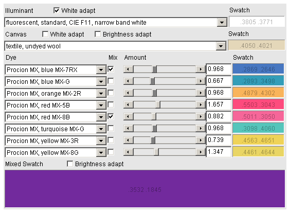
Here are descriptions of the different parts of the Dye Mixer user interface:

  • You can alter the virtual lighting conditions by choosing the appropriate Illuminant. Objects appear a different color under different illuminants, so make a choice similar to what you have where your work will be viewed in.
  • Illuminant Swatch shows the appearance of the illuminantion on a truly white surface. Each Swatch shows its CIE xy color coordinates.
  • Checking Illuminant White adapt makes the illumination appear the same color as the white on your computer screen, to which your vision has adapted to. This will make subjective color evaluation easier. However, if you want to compare absolute colors by holding an object against the computer screen, you should uncheck Illuminant White adapt.
  • Before proceeding to dyes, you must choose the Canvas. Dyes appear different color on different canvases.
  • Canvas Swatch shows the appearance of the canvas in the chosen illumination.
  • Checking Canvas White adapt makes the canvas appear the same color as the white on your computer screen. This may be useful if you have a large canvas, to which your vision adapts, and a small dyed area, and you want to see how the dyed area appears in the context of its surroundings. To view absolute colors, uncheck Canvas White adapt.
  • Checking Canvas Brightness adapt increases the amount of light the canvas is exposed to, but does not interfere with the absolute tone of color. Canvas Brightness adapt has no effect if Canvas White adapt is enabled.
  • The Dye Mixer allows mixing 8 dyes simultaneously. For each dye:
    • Choose the Dye you want to use. Note that the Dye Mixer is ignorant of the chemical compatibility of different dyes and canvases.
    • Checking Mix will include the dye in the combined mixture of dyes.
    • Amount of dye can be changed either by operating the slider, or numerically. The actual amount or concentration of dye required for the same effect in the laboratory can be direcly proportional to the Amount value. (I’d love to hear your experiments on this!) The proportionality coefficient you must use is different for different dyes and canvases.
    • Swatch shows the dyed canvas.
  • Mixed swatch shows the canvas dyed with all the selected dyes.
  • Checking Mixed swatch Brightness adapt increases the amount of light the dyed canvas is exposed to, but does not interfere with the absolute tone of color.

Here are some typical uses for the Dye Mixer:

  • You have a color in the back of your mind and wish to find a dye combination to realize it. Set your computer screen white balance so that it matches the white balance in the space you are in, or just let your eyes adjust to the monitor white balance. Enable Illuminant White adapt. Choose the Canvas and Illuminant as close as possible to what your work will be showed using. Try different dye amounts and combinations until you get an acceptable result. Just to be sure, write down what you are using. Try to use dyes sparingly! In actual reality, for each of the dyes you use in the mix, dye a swatch and see if it gets the same tone of color as the Dye Swatch in the Dye Mixer. Adjust the amount of dye until you have a matching result (see below for matching instructions).
  • You want to compare the color of a real-life object to a color produced by the Dye Mixer. Adjust the white balance of your computer screen to 6500 K. Choose an illuminant as close as possible to what you have in the space you are in. Disable white adaptations in the Dye Mixer. Adjust the computer screen contrast and the amout of lighting in your room so that the Dye Mixer’s swatch has the same brightness as the object. Compare the colors between the Dye Mixer’s swatch and the object.

Happy mixing!

Version history

This is version 1.1 of the Dye Mixer. Some of the older versions are available. The evolution of the Dye Mixer has been as follows (read from bottom to top):

1.1 Plenty of illuminant, canvas and dye data has been added. Most of the data is now in a separate text file, allowing adding new data without recompilation, or updating the Dye Mixer version. The biggest improvement, however, is that now the Dye Mixer is Java 1.1 compatible! This is good because Sun’s license for Java 1.2 (used in the Dye Mixer 1.0) and greater is, for some users and browser vendors, unacceptably restrictive. There has been some changes in the scalings of dye amounts – sorry about that if you wrote down some formulas. You can convert the 1.0 amounts to 1.1 notation by a simple calculation.
1.0 Added sliders and some minor things; improved much on ease of use.
0.9 Initial version.

Technical details

The jar package of the applet is made available for download.

The operation of Dye Mixer is spectrum-based. So, adding a new light source, canvas or dye will require measuring the spectrum. I will be happy to add a new dye (or light, or canvas) if you can provide me with its spectrum and as much information of the dye as possible. If you are unable to locate a spectrophotometer, you could also send me a sample of the dye.

The Procion MX dye absorbance spectra were measured with a spectrophotometer from 350 nm to 800 nm at 5 nm steps, using concentrations that kept absorbance under 1.0, with distilled water as solvent. The canvas reflectance spectra were measured with my own mirror apparatus combined with a spectrophotometer, using a tissue paper as white reference. The theoretical light spectra are computed by Dye Mixer and the rest of the spectra were obtained from various sources.

A simple absorbance model is used with the dyes: The absorbance spectrum of a dye is multiplied by the amount value. This is analogous to increasing the thickness, or concentration, of the dye layer. The model is unable to handle fluorescent materials and dyes.

The CIE XYZ tristimulus coordinates are calculated from the obtained light spectrum and further converted into sRGB for viewing. Java XYZ to sRGB conversion uses CIE D50 instead of CIE D65, so I coded my own according to the sRGB standard. sRGB uses the CIE D65 reference illuminant white point, so you should adjust your monitor and your room lighting to 6500 K color temperature, if you want to view absolute colors and compare samples directly against the picture on the monitor. Normally you should, however, resort to subjective comparison, using the screen white as the white reference for the virtual sample, and the room lighting (as reflected from white walls, paper) as the white referene for the actual sample.

References

The input spectra came from various sources:

  • CIE, standards spectra.
  • Wenham, S.R., Green, M.A. and Watt, M.E., standards spectra.
  • Mitsubishi Electric, illuminant spectra.
  • Kobus Barnard, Lindsay Martin, Brian Funt and Adam Coath, illuminant spectra.
  • Jouni Haanpalo, dye absorbance spectra.
  • Eastman Kodak, reflectance spectra.
  • Purdue University, reflectance spectra.
  • Noboru Ohta, reflectance spectra.

Links

Here are some related links:

A bit of background

I got interested in textile dyes after I bought a tie-dye T-shirt at Berkeley, California, which I visited during a “business trip” in spring 2001. I loved the place for it atmosphere, too. I grew fond of colorful hippie clothes, and wanted more. I could not find any locally (in Finland, they hardly even sell T-shirts during winter). The consequence was that I ordered, together with my mother Hanna (I didn’t have a credit card) some Procion MX dyes from Quilt und Art, Germany, to dye my own clothes.

Since, I have dyed tens of T-shirts and some other items. Most have been bought by my friends, for small fees certainly not to be of any interest to tax officials… :-)

Impulse response measurements

2006/08/10

To measure the impulse response of a noisy system, you don’t want to just send an impulse and see what comes out. Instead, you will play a signal that has succifiently high energy (long instead of loud), record the outcome and deconvolve from it your original signal, giving you the impulse response.

Golay codes

I measured these impulse responses from the home audio system of my friend Mikko Nelo at his city flat (check the pic for an overview. There might have been a subwoofer somewhere too, but I don’t remember…). Hehe, at least the bass is there. Miniature microphones were plugged into my ears, a minidisc recorder operated as a pre-amp and a laptop I borrowed from work as the player/recorder. A lengthy pair of Golay codes was used as the measurement signal because that way it was easy to deconvolve with existing tools. The following measurements are in binaural stereo 44100Hz 16bit WAV: ir_left.wav (158kB), ir_right.wav (112kB), ir_mono.wav (113kB). Here’s a piece of music unprocessed/processed to demonstrate the use of the impulse responses: irtest.mp3 (559kB). Headphones required!

Chirp signals

Any signal with a perfectly flat frequency content can be deconvolved by convolving with its reverse. Chirp signals (a.k.a. frequency sweeps) made using IFFT can be perfectly flat in the periodic signal sense. Here is such a 65536-sample chirp: chirp64k.wav (WARNING: SOUNDS NASTY). It can be used to analyze up to one second impulse responses. You must play the chirp signal in a loop a few times, record the result, deconvolve, and pick one of the middle impulse responses. Using this method, I have made inverse filters for headphones, which can be used for example with the RealReverb plugin for WinAmp.

Evolutionary real variable optimization in C++

2006/08/10

If you have a problem where you need to find the optimal values for a set of real variables, try this library written by Magnus Jonsson and me.


opti.cpp opti.hpp – Optimization library

MersenneTwister.h – Mersenne Twister random number generator required by the library (by Rick Wagner)

optitest.cpp keyboard.h – Example program with keyboard IO routines


Look at opti.hpp for the interfaces to the library. Read this text to know what is the idea of the various things and what can be done to improve the optimization.

You must present your optimization problem in form of a cost function that accepts a vector of parameters (real numbers) and gives out a single (real) number. The library will then try to find the combination of values for the parameters that minimizes the value your cost function. Sometimes a sub-optimal solution is found, but, depending on the hardness of the problem, often the global optimum is reached.

The basic idea of how an evolutionary algorithm works is as follows. First a population of parameter vectors is initialized to random values that cover the whole range of possible values for the optimal solution. Then the evolutionary algorithm will combine members of the population to create new trial vectors. The trial vectors may replace inferior members in the population. Ultimately, the population will dive into a minimum, hopefully the global minimum, of the cost function.

Different evolutionary strategies available in the library:

  • Differential evolution (class DE)

This algorithm adds scaled-down differences between population members to other population members to create trial vectors.

  • G3PCX (class G3, PCX is the default recombinator)

This algorithm is based on creating trial vectors randomly in the vicinity of existing population members. The extent of the randomness depends on the scattering of the population.

  • GreedyMagnus (class GreedyMagnus)

The name means it converges fast but may therefore get sucked into a local optimum.

In the library, the recombinator means the part of the evolutionary algorithm that combines population members to create the trial vectors. We made the library in a flexible way so that you can exchange the recombinators between the optimization strategies. A default recombinator is provided for each strategy, but some experimenting with the recombinator parameters may improve the reliability and the speed of the optimization, as different types of problems benefit from different approaches. The parameters in the recombinators are as follows.

  • DERecombinator

This recombinator is to be used with Differential Evolution. The parameter cr defines how many of the parameters from the trial vector will replace corresponding parameters in the inferior vector. Usually a value of 1 is OK, but if your population size is small, there is a danger that the dimensionality of your population might drop too low. A value of 0.999 will add a refreshing dash of randomness to the otherwise linear way of combining of the vectors, but will not disturb the over-all scheme too much. The parameter c is the number by which the difference between two population members is multiplied before it is added to another member to create the trial vector. Values such as 0.3, 0.4, 0.6, 0.7 and 0.8 have been useful.

  • PCXRecombinator

This recombinator is to be used with the G3 strategy. The parameter sd1 and sd2 are standard deviations of the random vectors that are created around existing population members, expressed relative to distances between randomly selected members of the populaton. It is fine to have the same value for both. 0.1 is a nice choice. You should normally stay under 1. A low number will make the population progress in smaller steps, thus better fine-tuning a found minimum, but a higher value will make the population explore more distant areas in the cost function. numparents means how many population members will be selected for the recombination process ecah time. 3 is the default value, which I haven’t found useful to change.

  • MagnusRecombinator

This recombinator has no adjustable parameters. It is to be used with GreedyMagnus.

The population size is something you must always define by yourself. Practical values are in the range of 30-1000, but even higher values might be used in over-night optimizations where you don’t want to take any chances. If the population is large enough to explore the cost function properly, the global minimum will be reached within a low numerical error. You should always use more population members than you have dimensions in your problem.

The optimization is advanced by repeated calling of the evolve() function, which advances the population somewhat (how many evaluations of the cost function it does depends on the implementation of the strategy) and returns the cost of the best parameter vector so far in the population. Also the average cost of the population can be quickly retrieved using the avarageCost() function. The optimization should be stopped when there is no more progress within the numerical accuracy that you require. The best vector in the population is returned by the function best(). Try to refrain from printing progress information on each iteration, or your program might be occupied mostly by the print function…
If many repeated runs of the optimization return the same solution, it is quite likely that you have reached the global minimum, because there are typically a huge number of local minima and if you are stuck at one, you probably won’t be stuck at the same the next time. Just look at the solved digits of the cost function value. These will work as a kind of fingerprint of the minimum. If you have problems getting into the global minimum or you are unsure that you are there, you may want to start with a similar problem but of a lower dimensionality. Then increase the dimensionality step by step. If you see a nice trend in the costs of the found solutions for each dimensionality, then this is an extra encouragement that you are at the global minimum.

To speed up things, reduce the running time of your cost function. If your cost function is a sum of a number of terms, then you can employ the compare variable passed to the cost function by the optimizer. If your cost seems to go above this value, then you can stop evaluation of the terms and just return compare or some larger number. This will instruct the optimizer that the evaluated trial vector is worse than another other vector it is comparing it against, and therefore can be discarded. (Note: GreedyMagnus will not speed up using this trick.) If you use this trick, then it makes sense to first evaluate terms you suspect will give the biggest penalty.

It is also possible to constrain the variables being optimized. You can do this by modifying the input vector at the beginning of the cost function. But carefully consider what might be the consequences of this modification. If you hard-limit some parameters, will this reduce the dimensionality of your population as you set a parameter to the same value in many of the vectors? It can be better to just penalize strongly solutions that go outside your bounds of choice, by adding a large penalty term. Perhaps even create a sort of a funnel in the cost function that will direct astray vectors back on track. This can be done by penalizing according to the severity of the constraint violation.

This is getting a bit problem-specific, but if you are doing something like least mean square approximation, you typically are integrating the error function through sampling. Do this so that you concentrate more samples at the known problem areas of the function. This way you can reduce the total number of samples significantly and will speed up the execution of the cost function.

Powered by WordPress - Hosted by SuniSoft oy