Skip to content
iki.fi/o
Category:
Computation
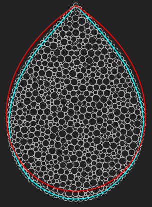
Teardrop simulation
For more info see this
Mathematics StackExchange post
with my reply.
Posts navigation
Page
1
Page
2
…
Page
13
Next page